Sensitivity analysis toolbox example - Ishigami
The model
The ishigami model has three parameters x1,x2,x3 with interactions between x1 and x3. Create the following expression Y in Ecolego.
y = sin(x1)+7.0*sin(x2)^2.0+0.1*x3^4.0*sin(x1)
Assign a uniform distributions unif(min=-3.14, max=3.14) to the parameters x1,x2,x3. Assign the parameters a value of 0.
Setting up the Sensitivity Analysis
Open the Sensitivity Analysis Toolbox perspective by clicking the button  in the ecolego toolbar.
When first entering the Sensitivity Analysis view, a message might be opened to request the simulation type be changed to Sensitivity Analysis. This is recommended to make errors and warnings be shown correctly.
Selection of probabilistic parameters
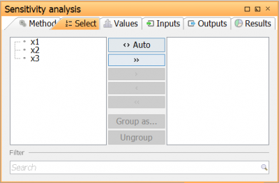 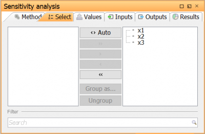 |
| Go to Select tab to open the Parameter selection view. Here, the parameters for which the sensitivity analysis should be run are selected. Select all three parameters x1,x2 and x3 by moving them to the right in the parameter selection view |
Selection of Sensitivity analysis method
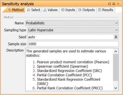 | Go to Method tab to open the Sensitivity analysis method view. Here, the sensitivity analysis method and its settings is selected. Select the method Probabilistic with the following settings: Sampling type: Latin Hypercube Seed: Auto Base sample size: 1000 |
Running the sensitivity analysis
When all appropriate settings has been set, the sensitivity analysis can be run. This is done in the following way:
First, the samples for each selected parameter is generated. The sample scheme is defined by the selected Sensitivity Analysis method. In this example, 1000 samples are generated with Latin hypercube independently for each of the parameters. For other methods, such as Sobol and EFAST, the sampling is not independent for the parameters, but follow specific rules.
Secondly, the model outputs are simulated using the generated parameter samples.
Thirdly, the sensitivity indices are calculated for a given output when a correlation chart or table is created.
Note: Step one and two can be done with one command (see Calculate and inspect the sensitivity analysis result), but here it is described how to do it in two steps.
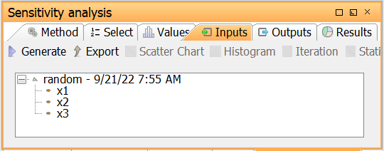
Generate parameter samples
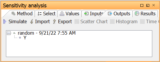
Simulate model outputs
| Calculate and inspect the sensitivity analysis result |
|---|
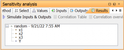 |
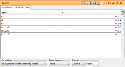
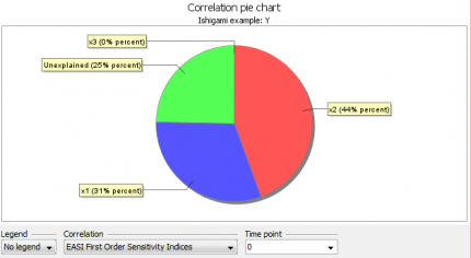
| Go to Results tab to open the Results view. Here, a shortcut is given to generate both inputs and outputs by clicking generate inputs & outputs. In this view, sensitivity and correlation measures can be inspected in charts and/or tables In the tree, select the only output y A Correlation table is created, showing the sensitivity indices for the parameters on the output. Here, the first order sensitivity indices (EASI) is approximately 30%, 44% and 0% for the parameters x1,x2 and x3 respectively. Select the output y and select Pie chart to create a Correlation Pie Chart for the first order indices. As seen in the chart and table, x1 and x2 has relatively large first order indices while x3 has a very small or zero first order index. However, it is also seen that the unexplained part is quite large (nearly 25%) which suggests effects which are not explained by the first order indices. Calculation of second order indices In the Correlation table, select XEASI as correlation measure. This measure calculates the second order indices between pairwise combinations of parameters. It is seen that there are second order indices which are relatively large (nearly 30% for x2). Note: Non zero higher order effects are resulting due to the limited number of samples. It is seen from the model expression that only x2 has a true non-zero interacting effect. |
  |
See also

