Sensitivity analysis toolbox example - Cow
Creating the model
This example uses a simple model of the uptake of lead in the milk and meat of a cow.
Create two expressions for the concentration of lead in beef (Cbeef) and milk (Cmilk) as follows:
Cbeef = TFbeef*(Fgrass*Cgrass+Fwater*0.001*Cwater+Fair*Cair)
Cmilk = TFmilk*(Fgrass*Cgrass+Fwater*0.001*Cwater+Fair*Cair)
Cbeef and Cmilk depends on the concentration in the surroundings (grass, air and water) which are here modelled as periodic functions. Create the following expressions in ecolego:
Cgrass = 1.0E-7-if(mod(time,365.0)>120.0&&mod(time,365.0) < 250.0 ,cos(time/234.0)*1.0E-7)
Cair = 1.0E-6+sin(time/365.0*2.0*pi)*1.0E-7
Cwater = 8.0E-7+(sin(time/365.0*2.0*pi)+cos(time/341.0)*0.3)*4.0E-7
The above expressions depends on uncertain parameters. Create the following Parameters in Ecolego:
| Name | Distribution | Value |
|---|---|---|
| TF_beef | logn(mean=0.0012,sd=1.0) | 0.0012 |
| TF_milk | logn(mean=7.5E-5,sd=1.0) | 7.5E-5 |
| F_grass | triang(min=58.5,max=71.5,mode=65.0) | 65.0 |
| F_water | triang(min=20.0,max=150.0,mode=48.0) | 48.0 |
| F_air | triang(min=75.0,max=250.0,mode=150.0) | 150.0 |
Opening the Sensitivity analysis perspective
Open the Sensitivity Analysis toolbox perspective by clicking  in the Ecolego toolbar
When first entering the Sensitivity Analysis view, a message might be opened to request the simulation type be changed to Sensitivity Analysis. This is recommended to make errors and warnings be shown correctly.
Selection of probabilistic parameters
 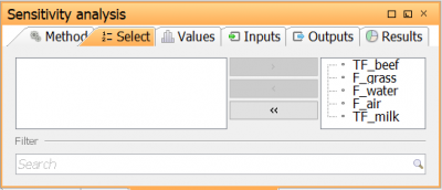 | Go to Select tab to open the Parameter selection view. Here, the parameters for which the sensitivity analysis should be run are selected. Select the five parameters in the table above by moving them to the right in the parameter selection view |
Selection of Sensitivity analysis method
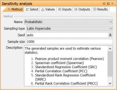 | Go to Method tab to open the Sensitivity analysis method view. Here, the sensitivity analysis method and its settings is selected. Select the method Probabilistic with the following settings: Base sample size: 1000 Sampling type: Latin Hypercube Calculate second order indices: Unchecked Seed: Auto |
Modification of parameter values (optional)
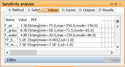 | Go to Values to open the Parameter values view. Here, the Parameter values can be reviewed and changed if necessary. Keep the values set earlier. |
Running the sensitivity analysis
When all appropriate settings has been set, the sensitivity analysis can be run. This is done in the following way:
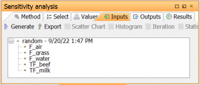
First, the samples for each selected parameter is generated. The sample scheme is defined by the selected Sensitivity Analysis method. In this example, 1000 samples are generated with Latin hypercube independently for each of the five parameters. For other methods, such as Sobol and EFAST, the sampling is not independent for the parameters, but follow specific rules.
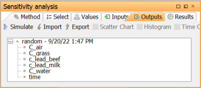
Secondly, the model outputs are simulated using the generated parameter samples.
Thirdly, the sensitivity indices are calculated for a given output when the output when a correlation chart or table is created.
Note: Step one and two can be done with one command (see Calculate and inspect the sensitivity analysis result), but here it is described how to do it in two steps.
Generate parameter samples
Simulate model outputs
Calculate and inspect the sensitivity analysis result

Go to the Results tab to show the Results view. Here, a shortcut is given to general both inputs and outputs by clicking generate inputs & outputs. In this view, sensitivity and correlation measures can be inspected in charts and/or tables
In the tree, select Cbeef and Cmilk
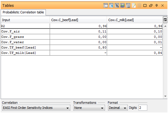
A Correlation table is created for the selected outputs, displaying the sensitivity indices calculated by the probabilistic method. Select the Transformation from the drop down list under the table and put it on Rank.
Now, select Cbeef and click Correlation pie chart
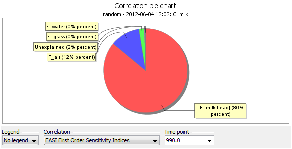
A Correlation pie chart is created and for Cmilk and displays the first order sensitivity index of all parameters on the selected output. The same can be done for Cbeef. Right click on the Chart and click on Edit. In the Data tab, select the Transformation and put it on Rank.
As seen in the chart and table, C_beef is most sensitive to TF_beef and C_milk the most sensitive to F_milk (both having a first order index of approximately 0.80. F_air also contribute a first order index of approximately 0.10. All other numbers are zero or very close to zero. The coefficient of determination R2 is close to 1 (0.96) and is an indication that the output samples are nearly linear in terms of the inputs samples. This implies that there should not be any significant contribution of higher order sensitivity indices (measuring interacting parameters). This conclusion is also supported by the very small (2%) unexplained part of the pie chart (for a perfect linear relationship, all first order sensitivity indices should sum to 1 leaving zero unexplained part).
See also

